Home » Articles » 23c » Here

SQL Property Graphs and SQL/PGQ in Oracle Database 23c

Oracle have had a Graph Server and Client product for some time, but in Oracle database 23c some of the property graph functionality has been built directly into the database.

This article focuses on new SQL property graph feature and ignores the previous Graph Server product and PGQL.

• Setup
• SQL Property Graphs
• SQL/PGQ (GRAPH_TABLE)
• Oracle Graph Visualization
• Query Transformation
• JSON Support

Setup

We create a new test user. We add a couple of extra privileges that allow us to do some tracing and display execution plans, but these are not necessary when using SQL property graphs.

conn sys/SysPassword1@//localhost:1521/freepdb1 as sysdba

drop user if exists testuser1 cascade;

create user testuser1 identified by testuser1 quota unlimited on users;
grant db_developer_role to testuser1;

-- Only used for tracing and execution plan examples.
grant alter session to testuser1;
grant select_catalog_role to testuser1;

We need to make sure our test user has the ability to create property graphs.

grant create property graph to testuser1;

We create a table to hold people, and a table to record the connections between those people.

conn testuser1/testuser1@//localhost:1521/freepdb1

drop table if exists sales purge;
drop table if exists products purge;
drop table if exists connections purge;
drop table if exists people purge;


create table people (
  person_id number primary key,
  name      varchar2(15)
);

insert into people (person_id, name)
values (1, 'Wonder Woman'),
       (2, 'Peter Parker'),
       (3, 'Jean Grey'),
       (4, 'Clark Kent'),
       (5, 'Bruce Banner');
commit;


create table connections (
  connection_id  number primary key,
  person_id_1    number,
  person_id_2    number,
  constraint connections_people_1_fk foreign key (person_id_1) references people (person_id),
  constraint connections_people_2_fk foreign key (person_id_2) references people (person_id)
);

create index connections_person_1_idx on connections (person_id_1);
create index connections_person_2_idx on connections (person_id_2);

insert into connections (connection_id, person_id_1, person_id_2)
values (1,  1, 2),
       (2,  1, 3),
       (3,  1, 4),
       (4,  2, 4),
       (5,  3, 1),
       (6,  3, 4),
       (7,  3, 5),
       (8,  4, 1),
       (9,  5, 1),
       (10, 5, 2),
       (11, 5, 3);
commit;

We create a table to hold products, and a table to hold sales, linked back to the people we defined earlier.

create table products (
  product_id  number primary key,
  name        varchar2(10)
);

insert into products (product_id, name)
values (1, 'apple'),
       (2, 'banana'),
       (3, 'lemon'),
       (4, 'lime');
commit;


create table sales (
  sale_id     number primary key,
  person_id   number,
  product_id  number,
  quantity    number,
  constraint sales_people_fk foreign key (person_id) references people (person_id),
  constraint sales_products_fk foreign key (product_id) references products (product_id)
);

create index sales_person_id_idx on sales (person_id);
create index sales_product_idx on sales (product_id);

insert into sales (sale_id, person_id, product_id, quantity)
values (1, 1, 2, 10),
       (2, 1, 3, 5),
       (3, 2, 2, 6),
       (4, 2, 1, 4),
       (5, 3, 2, 3),
       (6, 3, 1, 6),
       (7, 3, 3, 2),
       (8, 4, 3, 8),
       (9, 5, 2, 6),
       (10, 5, 4, 5),
       (11, 5, 3, 3);
commit;

We gather statistics on all the tables.

exec dbms_stats.gather_table_stats(null, 'people');
exec dbms_stats.gather_table_stats(null, 'connections');
exec dbms_stats.gather_table_stats(null, 'products');
exec dbms_stats.gather_table_stats(null, 'sales');

SQL Property Graphs

A property graph is a model that describes nodes (vertices), and the relationships between them (edges). In the case of SQL property graphs introduced in Oracle database 23c, the vertices and edges are schema objects such as tables, external tables, materialized views or synonyms to these objects. The property graph is stored in the database, and can be referenced by SQL/PGQ queries. There is no data materialized by the SQL property graph, it is just metadata. All the actual data comes from the references objects.

We create a property graph where the PEOPLE table represents the vertices (the points) and the CONNECTIONS table represents the edges (the lines between the points).

--drop property graph connections_pg;

create property graph connections_pg
  vertex tables (
    people
      key (person_id)
      label person
      properties all columns
  )
  edge tables (
    connections
      key (connection_id)
      source key (person_id_1) references people (person_id)
      destination key (person_id_2) references people (person_id)
      label connection
      properties all columns
  );

The LABEL keyword allows us to associate a meaningful name, which we can reference in queries. Notice the edge table has a SOURCE KEY and DESTINATION KEY describing the connection between the vertices.

We create a property graph for the sales of products to people. The vertex tables are PEOPLE and PRODUCTS, and the edge table is SALES.

--drop property graph sales_pg;

create property graph sales_pg
  vertex tables (
    people
      key (person_id)
      label person
      properties all columns,
    products
      key (product_id)
      label product
      properties all columns
  )
  edge tables (
    sales
      key (sale_id)
      source key (person_id) references people (person_id)
      destination key (product_id) references products (product_id)
      label sale
      properties all columns
  );

We display the current property graphs using the USER_PROPERTY_GRAPHS view.

column graph_name format a20
column graph_mode format a10
column allows_mixed_types format a17
column inmemory format a8

select * from user_property_graphs;

GRAPH_NAME           GRAPH_MODE ALLOWS_MIXED_TYPE INMEMORY
-------------------- ---------- ----------------- --------
CONNECTIONS_PG       TRUSTED    NO                NO
SALES_PG             TRUSTED    NO                NO

SQL>

SQL/PGQ (GRAPH_TABLE)

With the property graphs in place we can use the GRAPH_TABLE operator to query the property graphs using SQL/PGQ. We display people who are connected to each other.

select person1, person2
from   graph_table (connections_pg
         match
         (p1 is person) -[c is connection]-> (p2 is person)
         columns (p1.name as person1,
                  p2.name as person2)
       )
order by 1;

PERSON1         PERSON2
--------------- ---------------
Bruce Banner    Wonder Woman
Bruce Banner    Peter Parker
Bruce Banner    Jean Grey
Clark Kent      Wonder Woman
Jean Grey       Clark Kent
Jean Grey       Wonder Woman
Jean Grey       Bruce Banner
Peter Parker    Clark Kent
Wonder Woman    Clark Kent
Wonder Woman    Peter Parker
Wonder Woman    Jean Grey

11 rows selected.

SQL>

Let's break this query down.

• We call GRAPH_TABLE passing the property graph.
• We define the graph element pattern in the MATCH clause using the vertex and edge labels to show our relationship.
• We define the COLUMNS that will be available in our select list.

The MATCH clause elements can include a WHERE clause to limit the rows, and of course we can include a WHERE clause in the main body of the query.

select person1, person2
from   graph_table (connections_pg
         match
         (p1 is person where p1.name = 'Jean Grey') -[c is connection]-> (p2 is person)
         columns (p1.name as person1,
                  p2.name as person2)
       )
order by 1;

PERSON1         PERSON2
--------------- ---------------
Jean Grey       Wonder Woman
Jean Grey       Clark Kent
Jean Grey       Bruce Banner

SQL>


select person1, person2
from   graph_table (connections_pg
         match
         (p1 is person where p1.name = 'Jean Grey') -[c is connection]-> (p2 is person)
         columns (p1.name as person1,
                  p2.name as person2)
       )
where  person2 = 'Clark Kent'
order by 1;

PERSON1               PERSON2
--------------------- ---------------------
Jean Grey             Clark Kent

SQL>

To display the graph using Oracle Graph Visualization we need to include the VERTEX_ID and EDGE_ID functions to identify the IDs of the vertices and edges. These produce a fully qualified description of the element. In the following example we return a single row containing these values.

column id_p1 format a20
column id_c format a20
column id_p2 format a20
set linesize 200 pagesize 100

select person1, person2, id_p1, id_c, id_p2
from   graph_table (connections_pg
         match
         (p1 is person) -[c is connection]-> (p2 is person)
         columns (p1.name as person1,
                  p2.name as person2,
                  vertex_id(p1) AS id_p1,
                  edge_id(c) AS id_c,
                  vertex_id(p2) AS id_p2)
       )
where  rownum = 1
order by 1;

PERSON1         PERSON2         ID_P1                ID_C                 ID_P2
--------------- --------------- -------------------- -------------------- --------------------
Wonder Woman    Peter Parker    {"GRAPH_OWNER":"TEST {"GRAPH_OWNER":"TEST {"GRAPH_OWNER":"TEST
                                USER1","GRAPH_NAME": USER1","GRAPH_NAME": USER1","GRAPH_NAME":
                                "CONNECTIONS_PG","EL "CONNECTIONS_PG","EL "CONNECTIONS_PG","EL
                                EM_TABLE":"PEOPLE"," EM_TABLE":"CONNECTIO EM_TABLE":"PEOPLE","
                                KEY_VALUE":{"PERSON_ NS","KEY_VALUE":{"CO KEY_VALUE":{"PERSON_
                                ID":1}}              NNECTION_ID":1}}     ID":2}}


SQL>

This example uses our second property graph, and allows us to see people who are related by purchasing the same items.

select person1, product, person2
from   graph_table (sales_pg
         match
         (p1 is person) -[s1 is sale]-> (pr is product) <-[s2 is sale]- (p2 is person)
         columns (p1.name as person1,
                  p2.name as person2,
                  pr.name as product)
       )
where  person1 != person2
order by 1;

PERSON1         PRODUCT    PERSON2
--------------- ---------- ---------------
Bruce Banner    lemon      Jean Grey
Bruce Banner    banana     Jean Grey
Bruce Banner    banana     Peter Parker
Bruce Banner    lemon      Clark Kent
Bruce Banner    banana     Wonder Woman
Bruce Banner    lemon      Wonder Woman
Clark Kent      lemon      Bruce Banner
Clark Kent      lemon      Jean Grey
Clark Kent      lemon      Wonder Woman
Jean Grey       banana     Peter Parker
Jean Grey       apple      Peter Parker
Jean Grey       lemon      Wonder Woman
Jean Grey       banana     Wonder Woman
Jean Grey       lemon      Bruce Banner
Jean Grey       banana     Bruce Banner
Jean Grey       lemon      Clark Kent
Peter Parker    banana     Jean Grey
Peter Parker    banana     Wonder Woman
Peter Parker    apple      Jean Grey
Peter Parker    banana     Bruce Banner
Wonder Woman    banana     Jean Grey
Wonder Woman    lemon      Jean Grey
Wonder Woman    lemon      Bruce Banner
Wonder Woman    lemon      Clark Kent
Wonder Woman    banana     Peter Parker
Wonder Woman    banana     Bruce Banner

26 rows selected.

SQL>

As before, we need to include the IDs of the vertices and edges if we want to visualize the graph.

select person1, product, person2, id_p1, id_s1, id_pr, id_s2, id_p2
from   graph_table (sales_pg
         match
         (p1 is person) -[s1 is sale]-> (pr is product) <-[s2 is sale]- (p2 is person)
         columns (p1.name as person1,
                  p2.name as person2,
                  pr.name as product,
                  vertex_id(p1) AS id_p1,
                  edge_id(s1) AS id_s1,
                  vertex_id(pr) AS id_pr,
                  edge_id(s2) AS id_s2,
                  vertex_id(p2) AS id_p2)
       )
where  person1 != person2
order by 1;

Oracle Graph Visualization

There are several ways to deploy the Oracle Graph Visualization tool. In this case we deployed it using Tomcat.

Click on the "Oracle Graph Client" link here, and select the architecture you require. In this case we downloaded "Oracle Graph Webapps 23.2.0 for (Linux x86-64)". The SQL/PGQ support was added to the visualizer in version 23.1, so make sure you are not using an older version.

On the Tomcat server we did the following.

cd /tmp
unzip -oq V1033696-01-linux-webapps.zip
unzip -oq oracle-graph-webapps-23.1.0.zip
cp graphviz-23.2.0-tomcat.war $CATALINA_BASE/webapps/

We were then able to access the visualizer on the following URL.

https://localhost:8443/graphviz-23.2.0-tomcat

We log in with the following details.

Username: testuser1
Password: testuser1
Advanced > Database: jdbc:oracle:thin:@//localhost:1521/freepdb1

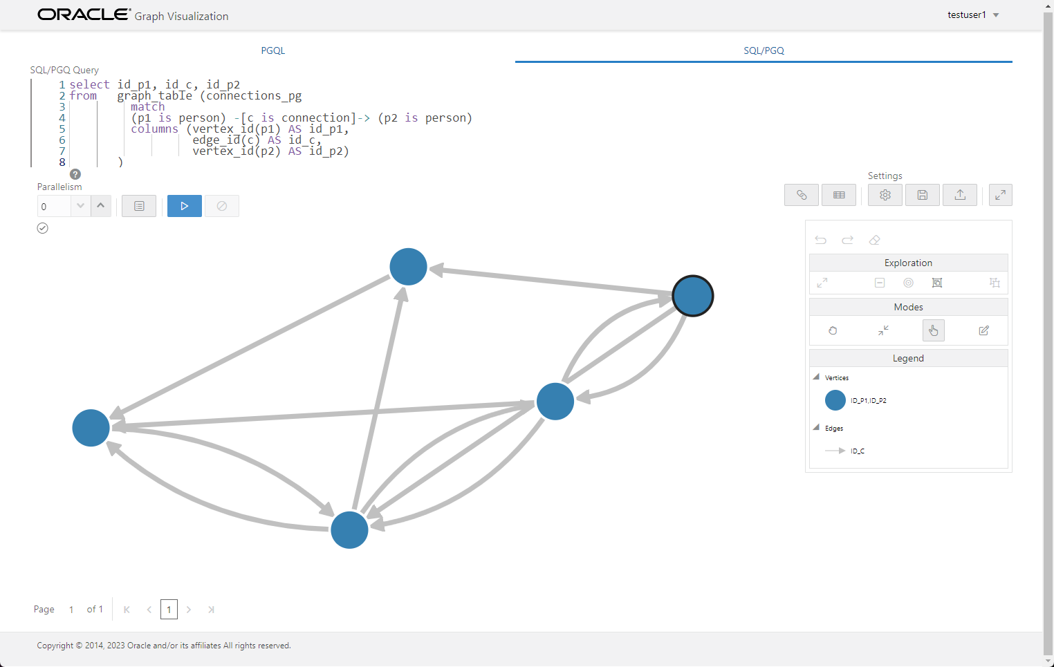
We click on the "SQL/PGQ" tab and place the following query into the visualizer. Notice it is missing the trailing ";". This query displays the connections between people.

select id_p1, id_c, id_p2
from   graph_table (connections_pg
         match
         (p1 is person) -[c is connection]-> (p2 is person)
         columns (vertex_id(p1) AS id_p1,
                  edge_id(c) AS id_c,
                  vertex_id(p2) AS id_p2)
       )

When we run it we get the following output.

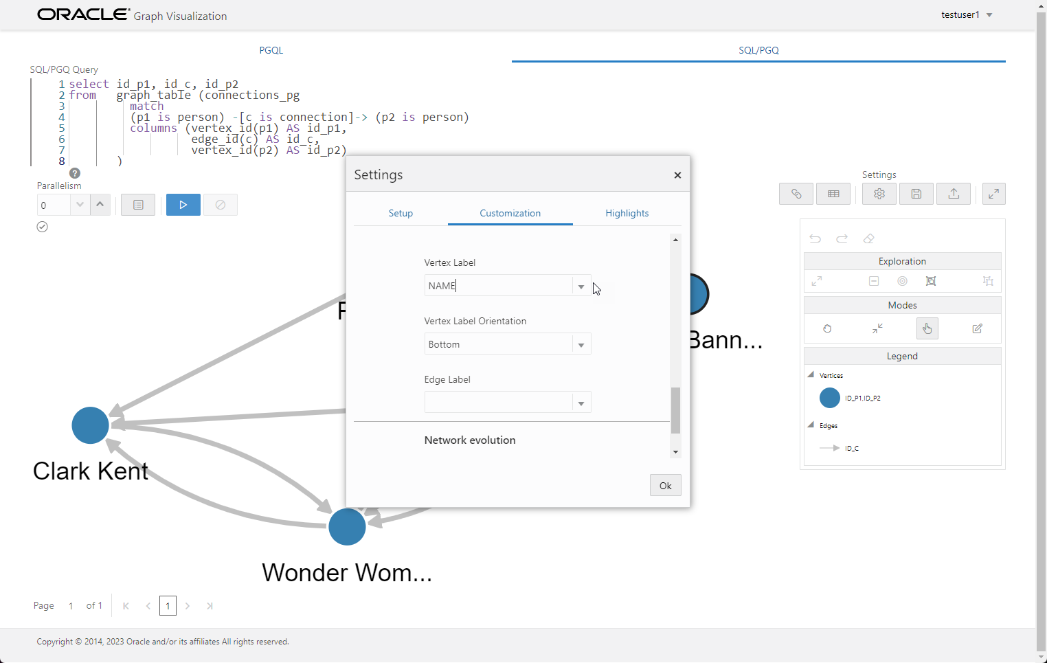
We click the settings (cog) button, click the "Customizations" tab, and set the "Vertex Label" to the NAME column.

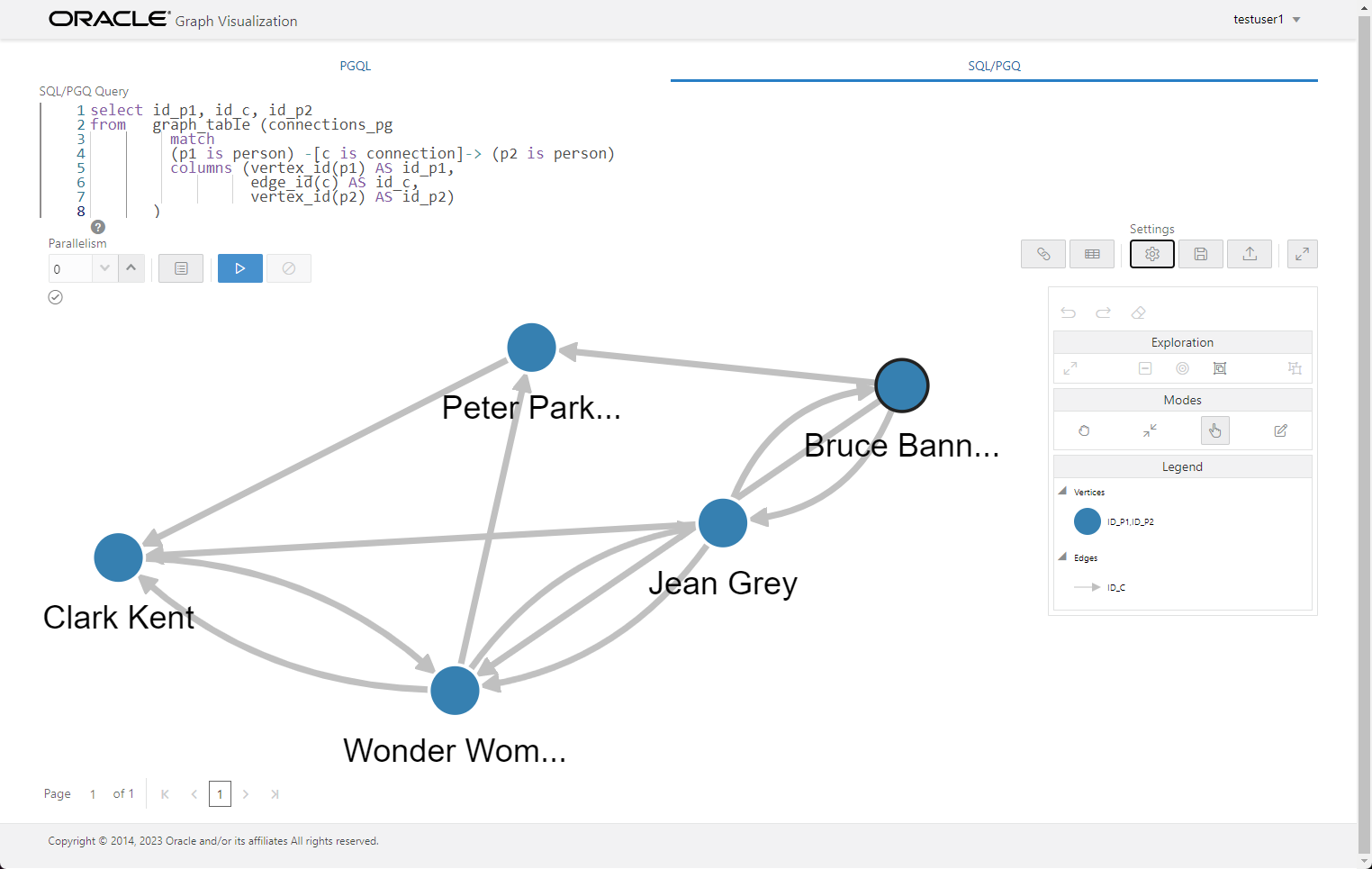
Once we click "OK" we see the graph with the labels.

We use the following query against our second property graph to shows the people who have purchased the same products.

select id_p1, id_s1, id_pr, id_s2, id_p2
from   graph_table (sales_pg
         match
         (p1 is person) -[s1 is sale]-> (pr is product) <-[s2 is sale]- (p2 is person)
         columns (p1.name as person1,
                  p2.name as person2,
                  vertex_id(p1) AS id_p1,
                  edge_id(s1) AS id_s1,
                  vertex_id(pr) AS id_pr,
                  edge_id(s2) AS id_s2,
                  vertex_id(p2) AS id_p2)
       )
where  person1 != person2

We run the query. In the "Customizations" tab we set the "Vertex Label" to NAME and the "Edge Label" to QUANTITY.

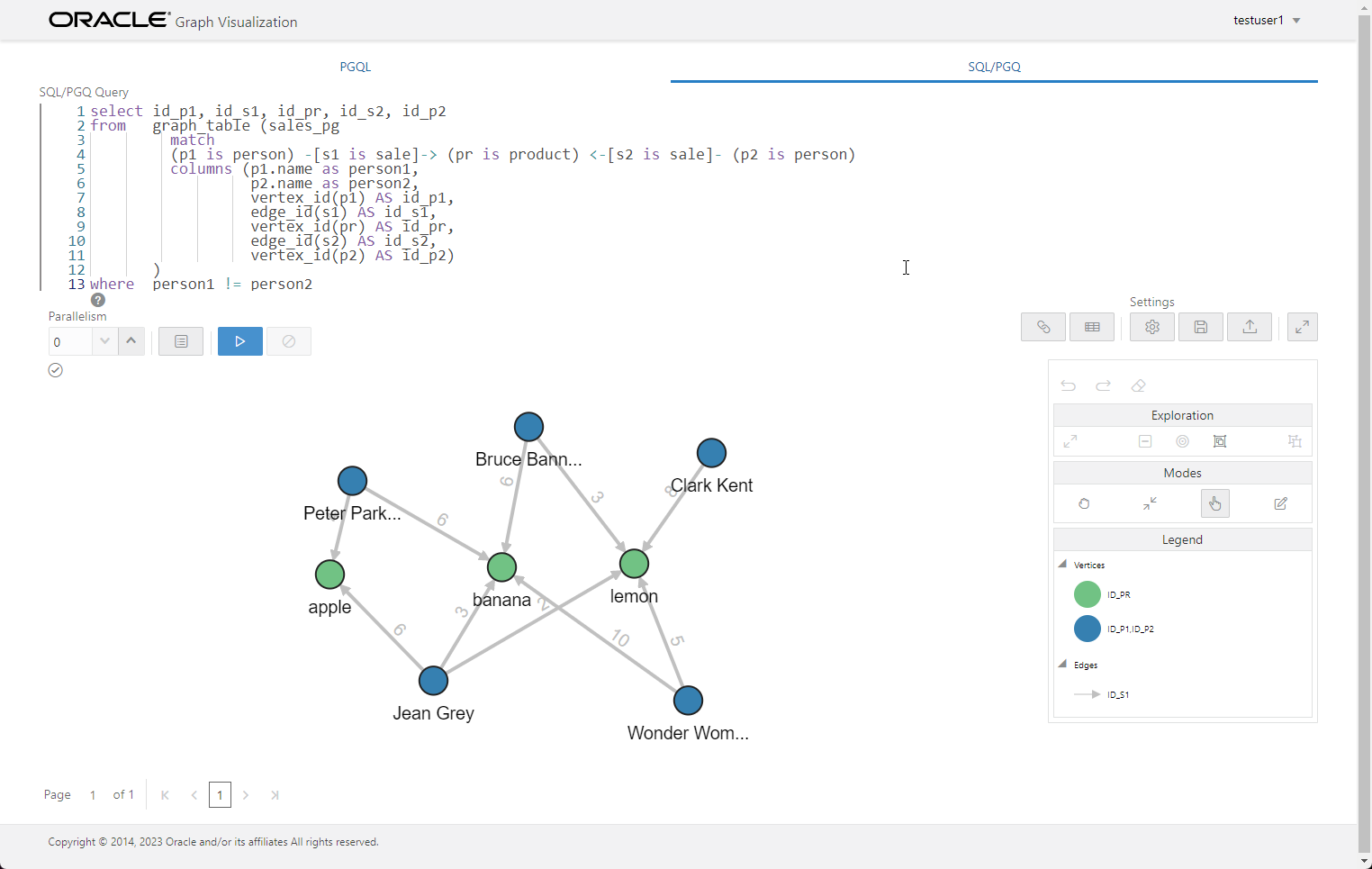
Not only can we see the relationship between the people and the products, but we can also see the quantity of the products purchased on the edge labels.

Query Transformation

Let's see what happens behind the scenes when we use SQL/PGQ.

First we flush the shared pool and identify the trace file that will be created for our new session.

conn sys/SysPassword1@//localhost:1521/freepdb1 as sysdba

alter system flush shared_pool;


conn testuser1/testuser1@//localhost:1521/freepdb1

set linesize 100
column value format a65

select value
from   v$diag_info
where  name = 'Default Trace File';

VALUE
-----------------------------------------------------------------
/opt/oracle/diag/rdbms/free/FREE/trace/FREE_ora_14020.trc

SQL>

Now we do a 10053 trace of the statement.

alter session set events '10053 trace name context forever';

select person1, product, person2
from   graph_table (sales_pg
         match
         (p1 is person) -[s1 is sale]-> (pr is product) <-[s2 is sale]- (p2 is person)
         columns (p1.name as person1,
                  p2.name as person2,
                  pr.name as product)
       )
where  person1 != person2
order by 1;

alter session set events '10053 trace name context off';

We check the resulting trace file, searching for the section beginning with "Final query after transformations", and we see the following statement.

Final query after transformations:******* UNPARSED QUERY IS *******
SELECT "P1"."NAME" "PERSON1",
       "PR"."NAME" "PRODUCT",
       "P2"."NAME" "PERSON2"
FROM   "TESTUSER1"."PEOPLE" "P1",
       "TESTUSER1"."SALES" "S1",
       "TESTUSER1"."PRODUCTS" "PR",
       "TESTUSER1"."SALES" "S2",
       "TESTUSER1"."PEOPLE" "P2"
WHERE  "P1"."NAME"<>"P2"."NAME"
AND    "P1"."PERSON_ID"="S1"."PERSON_ID"
AND    "PR"."PRODUCT_ID"="S1"."PRODUCT_ID"
AND    "P2"."PERSON_ID"="S2"."PERSON_ID"
AND    "PR"."PRODUCT_ID"="S2"."PRODUCT_ID"
ORDER BY "P1"."NAME"

The statement has been transformed to convert the SQL/PGQ into regular joins. In this example there is not a great deal of difference in complexity between the SQL/PGQ and the transformed SQL statement, but in some scenarios the SQL/PGQ can massively simplify the joins and unions necessary to return the data.

Since the SQL/PGQ is converted to regular SQL, it's possible to display the execution plan in the normal way.

select person1, product, person2
from   graph_table (sales_pg
         match
         (p1 is person) -[s1 is sale]-> (pr is product) <-[s2 is sale]- (p2 is person)
         columns (p1.name as person1,
                  p2.name as person2,
                  pr.name as product)
       )
where  person1 != person2
order by 1;


select * from table(dbms_xplan.display_cursor(format=>'ALL'));

PLAN_TABLE_OUTPUT
------------------------------------------------------------------------------------------------------------------------
SQL_ID  2j4yv6j0gks9y, child number 0
-------------------------------------
select person1, product, person2 from   graph_table (sales_pg
match          (p1 is person) -[s1 is sale]-> (pr is product) <-[s2 is
sale]- (p2 is person)          columns (p1.name as person1,
      p2.name as person2,                   pr.name as product)
) where  person1 != person2 order by 1

Plan hash value: 3808001794

--------------------------------------------------------------------------------------------------------
| Id  | Operation                        | Name                | Rows  | Bytes | Cost (%CPU)| Time     |
--------------------------------------------------------------------------------------------------------
|   0 | SELECT STATEMENT                 |                     |       |       |    14 (100)|          |
|   1 |  SORT ORDER BY                   |                     |    24 |  1224 |    14  (15)| 00:00:01 |
|*  2 |   HASH JOIN                      |                     |    24 |  1224 |    13   (8)| 00:00:01 |
|*  3 |    HASH JOIN                     |                     |    30 |  1080 |    10  (10)| 00:00:01 |
|*  4 |     HASH JOIN                    |                     |    11 |   330 |     8  (13)| 00:00:01 |
|   5 |      MERGE JOIN                  |                     |    11 |   165 |     5  (20)| 00:00:01 |
|   6 |       TABLE ACCESS BY INDEX ROWID| PRODUCTS            |     4 |    36 |     2   (0)| 00:00:01 |
|   7 |        INDEX FULL SCAN           | SYS_C0012556        |     4 |       |     1   (0)| 00:00:01 |
|*  8 |       SORT JOIN                  |                     |    11 |    66 |     3  (34)| 00:00:01 |
|   9 |        VIEW                      | index$_join$_003    |    11 |    66 |     2   (0)| 00:00:01 |
|* 10 |         HASH JOIN                |                     |       |       |            |          |
|  11 |          INDEX FAST FULL SCAN    | SALES_PERSON_ID_IDX |    11 |    66 |     1   (0)| 00:00:01 |
|  12 |          INDEX FAST FULL SCAN    | SALES_PRODUCT_IDX   |    11 |    66 |     1   (0)| 00:00:01 |
|  13 |      TABLE ACCESS FULL           | PEOPLE              |     5 |    75 |     3   (0)| 00:00:01 |
|  14 |     VIEW                         | index$_join$_005    |    11 |    66 |     2   (0)| 00:00:01 |
|* 15 |      HASH JOIN                   |                     |       |       |            |          |
|  16 |       INDEX FAST FULL SCAN       | SALES_PERSON_ID_IDX |    11 |    66 |     1   (0)| 00:00:01 |
|  17 |       INDEX FAST FULL SCAN       | SALES_PRODUCT_IDX   |    11 |    66 |     1   (0)| 00:00:01 |
|  18 |    TABLE ACCESS FULL             | PEOPLE              |     5 |    75 |     3   (0)| 00:00:01 |
--------------------------------------------------------------------------------------------------------

Query Block Name / Object Alias (identified by operation id):
-------------------------------------------------------------

   1 - SEL$E6D2A9F4
   6 - SEL$E6D2A9F4 / "PR"@"SEL$88741CE7"
   7 - SEL$E6D2A9F4 / "PR"@"SEL$88741CE7"
   9 - SEL$2237A74B / "S1"@"SEL$88741CE7"
  10 - SEL$2237A74B
  11 - SEL$2237A74B / "indexjoin$_alias$_001"@"SEL$2237A74B"
  12 - SEL$2237A74B / "indexjoin$_alias$_002"@"SEL$2237A74B"
  13 - SEL$E6D2A9F4 / "P1"@"SEL$88741CE7"
  14 - SEL$37BF1F62 / "S2"@"SEL$88741CE7"
  15 - SEL$37BF1F62
  16 - SEL$37BF1F62 / "indexjoin$_alias$_001"@"SEL$37BF1F62"
  17 - SEL$37BF1F62 / "indexjoin$_alias$_002"@"SEL$37BF1F62"
  18 - SEL$E6D2A9F4 / "P2"@"SEL$88741CE7"

Predicate Information (identified by operation id):
---------------------------------------------------

   2 - access("P2"."PERSON_ID"="S2"."PERSON_ID")
       filter("P1"."NAME"<>"P2"."NAME")
   3 - access("PR"."PRODUCT_ID"="S2"."PRODUCT_ID")
   4 - access("P1"."PERSON_ID"="S1"."PERSON_ID")
   8 - access("PR"."PRODUCT_ID"="S1"."PRODUCT_ID")
       filter("PR"."PRODUCT_ID"="S1"."PRODUCT_ID")
  10 - access(ROWID=ROWID)
  15 - access(ROWID=ROWID)

Column Projection Information (identified by operation id):
-----------------------------------------------------------

   1 - (#keys=1) "P1"."NAME"[VARCHAR2,15], "PR"."NAME"[VARCHAR2,10], "P2"."NAME"[VARCHAR2,15]
   2 - (#keys=1) "P1"."NAME"[VARCHAR2,15], "PR"."NAME"[VARCHAR2,10], "P1"."NAME"[VARCHAR2,15],
       "P2"."NAME"[VARCHAR2,15], "P2"."NAME"[VARCHAR2,15]
   3 - (#keys=1) "P1"."NAME"[VARCHAR2,15], "PR"."NAME"[VARCHAR2,10], "P1"."NAME"[VARCHAR2,15],
       "S2"."PERSON_ID"[NUMBER,22]
   4 - (#keys=1) "PR"."PRODUCT_ID"[NUMBER,22], "PR"."NAME"[VARCHAR2,10],
       "P1"."NAME"[VARCHAR2,15], "P1"."NAME"[VARCHAR2,15]
   5 - "PR"."PRODUCT_ID"[NUMBER,22], "PR"."NAME"[VARCHAR2,10], "S1"."PERSON_ID"[NUMBER,22]
   6 - "PR"."PRODUCT_ID"[NUMBER,22], "PR"."NAME"[VARCHAR2,10]
   7 - "PR".ROWID[ROWID,10], "PR"."PRODUCT_ID"[NUMBER,22]
   8 - (#keys=1) "S1"."PRODUCT_ID"[NUMBER,22], "S1"."PERSON_ID"[NUMBER,22]
   9 - "S1"."PRODUCT_ID"[NUMBER,22], "S1"."PERSON_ID"[NUMBER,22]
  10 - (#keys=1) "S1"."PERSON_ID"[NUMBER,22], "S1"."PRODUCT_ID"[NUMBER,22]
  11 - ROWID[ROWID,10], "S1"."PERSON_ID"[NUMBER,22]
  12 - ROWID[ROWID,10], "S1"."PRODUCT_ID"[NUMBER,22]
  13 - "P1"."PERSON_ID"[NUMBER,22], "P1"."NAME"[VARCHAR2,15]
  14 - "S2"."PRODUCT_ID"[NUMBER,22], "S2"."PERSON_ID"[NUMBER,22]
  15 - (#keys=1) "S2"."PERSON_ID"[NUMBER,22], "S2"."PRODUCT_ID"[NUMBER,22]
  16 - ROWID[ROWID,10], "S2"."PERSON_ID"[NUMBER,22]
  17 - ROWID[ROWID,10], "S2"."PRODUCT_ID"[NUMBER,22]
  18 - "P2"."PERSON_ID"[NUMBER,22], "P2"."NAME"[VARCHAR2,15]

Note
-----
   - this is an adaptive plan


92 rows selected.

SQL>

JSON Support

In the previous examples we used PROPERTIES ALL COLUMNS to keep things simple. We could have limited the properties to specific table columns using a comma-separated list, as shown below.

--drop property graph connections_pg;

create property graph connections_pg
  vertex tables (
    people
      key (person_id)
      label person
      properties (name)
  )
  edge tables (
    connections
      key (connection_id)
      source key (person_id_1) references people (person_id)
      destination key (person_id_2) references people (person_id)
      label connection
      properties (person_id_1, person_id_2)
  );

Where we have columns containing JSON data, we can drill down into the JSON data using dot notation, or SQL/JSON function calls to define properties.

We add a JSON column to the PEOPLE table and populate it with some JSON data.

alter table people add (json_data json);


update people
set    json_data = json('{"gender":"female", "universe":"DC"}')
where  person_id = 1;

update people
set    json_data = json('{"gender":"male", "universe":"Marvel"}')
where  person_id = 2;

update people
set    json_data = json('{"gender":"female", "universe":"DC"}')
where  person_id = 3;

update people
set    json_data = json('{"gender":"male", "universe":"Marvel"}')
where  person_id = 4;

update people
set    json_data = json('{"gender":"male", "universe":"Marvel"}')
where  person_id = 5;

commit;

We recreate the property graph including the two new properties using an example of dot notation and a JSON_VALUE call.

drop property graph connections_pg;

create property graph connections_pg
  vertex tables (
    people
      key (person_id)
      label person
      properties (name,
                  people.json_data.gender.string() as gender,
                  json_value(people.json_data, '$.universe') as universe)
  )
  edge tables (
    connections
      key (connection_id)
      source key (person_id_1) references people (person_id)
      destination key (person_id_2) references people (person_id)
      label connection
      properties (person_id_1, person_id_2)
  );

We project the new properties as columns and add them into our select list.

column gender1 format a10
column gender2 format a10
column universe1 format a10
column universe2 format a10

select person1, gender1, universe1, person2, gender2, universe2
from   graph_table (connections_pg
         match
         (p1 is person) -[c is connection]-> (p2 is person)
         columns (p1.name as person1,
                  p1.gender as gender1,
                  p1.universe as universe1,
                  p2.name as person2,
                  p2.gender as gender2,
                  p2.universe as universe2)
       )
order by 1;

PERSON1         GENDER1    UNIVERSE1  PERSON2         GENDER2    UNIVERSE2
--------------- ---------- ---------- --------------- ---------- ----------
Bruce Banner    male       Marvel     Peter Parker    male       Marvel
Bruce Banner    male       Marvel     Wonder Woman    female     DC
Bruce Banner    male       Marvel     Jean Grey       female     DC
Clark Kent      male       Marvel     Wonder Woman    female     DC
Jean Grey       female     DC         Wonder Woman    female     DC
Jean Grey       female     DC         Clark Kent      male       Marvel
Jean Grey       female     DC         Bruce Banner    male       Marvel
Peter Parker    male       Marvel     Clark Kent      male       Marvel
Wonder Woman    female     DC         Clark Kent      male       Marvel
Wonder Woman    female     DC         Jean Grey       female     DC
Wonder Woman    female     DC         Peter Parker    male       Marvel

11 rows selected.

SQL>

For more information see:

• SQL Property Graphs
• Graph Developer's Guide for Property Graph
• CREATE PROPERTY GRAPH

Hope this helps. Regards Tim...

Back to the Top.

Created: 2023-06-02  Updated: 2023-06-19

Contact Us

Home | Articles | Scripts | Blog | Certification | Videos | Misc | About

About Tim Hall
Copyright & Disclaimer