8i | 9i | 10g | 11g | 12c | 13c | 18c | 19c | 21c | 23c | Misc | PL/SQL | SQL | RAC | WebLogic | Linux
Partitioning From a Design Perspective (A Practical Guide) - By Lothar Flatz
This is a guest post by Lothar Flatz. It is an English translation of an article first published in German here.
- Introduction
- Partitioning: a Definition
- Partitioning types and typical applications
- Conclusions
- About The Author
Introduction
It was the beginning of the 90s and I was working for the IT department of an international corporation when unexpectedly our users called. They asked if we had a server crash. A quick analysis revealed that a newly built data warehouse was the cause of the problems. The data warehouse was operated by another department in a neighbouring town. We sent the following message to our colleagues from the data warehouse development: "whatever you are doing right now, please stop it immediately". I was given the task of investigating what went wrong. I found that the colleagues were working on a sales statistics report. One of the search criteria was the current year. Unfortunately, there was an index on the Year column. The Rule based Optimizer considered using the index as the best option (unique comparison on single column index, rank 9). Therefore, over a million records of sales statistics were read one record at a time. Much better would have been a full table scan. However, this was out of the question for the Rule based Optimizer (full Table Scan, rank 15). With the advent of data warehouse applications, the character of database usage had changed fundamentally. New questions arose. For example "how to manage large amounts of data efficiently?" or "how to read a constrained number of rows with a full table scan?". Very soon the Rule based Optimizer was replaced to meet the new requirements. New data processing strategies had to be developed. One of the most important ways to process large amounts of data efficiently is partitioning. We will discuss the most important types of partitioning in this text.
It is the aim of this text to show typical solution patterns on the basis of practical examples and thus to stimulate the imagination of database designers in the direction of their own solution, rather than providing a complete overview of syntax and partitioning options.
Partitioning: a Definition
In this article we focus on horizontal partitioning [2].
The type of partitioning is essentially determined by three key elements.
- The distribution of data
- A rule that organizes the distribution
- A behaviour of the database engine that reflects the rule
Basically the documentation mentions three reasons for partitioning [1]:
The distribution of data
The data is divided into partitions. Essentially, a partition is nothing more than a table. Only that it is interpreted differently by the database engine.
A rule that organizes the distribution
There are many different ways to distribute data in partitions. There is always a key value (Partition Key) which decides by means of the rule in which partition a data record is stored. The rule can be a division into sorted ranges (Range Partitioning), or a mathematically evenly distributing function (Hash Partitioning), an assignment of single values (List Partitioning) or analogous to another table (reference Partitioning). To these basic possibilities there are then still variants like combinations (composite Partitioning) or administration simplifications (Interval Partitioning). The later two are not discussed here.
A behaviour of the database engine that reflects the rule
Depending on the type of partitioning, the database reacts differently to the individual partitioning variants. However, there are also some patterns common for all partitioning types. An example for this is the partition pruning. Here the optimizer exploits the search conditions of a query to compute which partitions the query must scan. Another type of general behaviour related to partitioning is, for example, that some basic manipulations of the table definition considers all partitions to be a unit. For example, if one drops a partitioned table, all partitions are dropped as a consequence.
Acceleration of access
This is the prime reason for partitioning. Via partition pruning it is possible to search specifically for data of a partition and at the same time to use the efficient Full Table Scan (here actually a Full Partition Scan). With the Full Table Scan all blocks of a table are read as they are stored. This makes it possible to read several blocks at once. Usually 128 blocks are read at once. How big is the improvement compared to single block reads? This depends on many details and varies a lot. To give you some idea though I add an example below. In order to do something sizable, I did a count over 100 million rows. As you can see, the multi block read is about 40 times faster. The result varies greatly depending on the task, but the Multi Block Read is clearly more efficient than an index scan when large amounts of data are to be read. A rule of thumb says that an index access is only worthwhile if 5% or less of the records of a table should be retrieved.
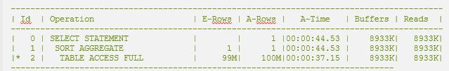
Listing 1: a full table scan which always means Multi Block Read
The next listing shows the same SQL with a single block read enforced via Hint. (An index scan is practically always a single block read. There are subvariants of it that do not change anything substantial. But the listing below is a classic case). As you can see the time difference is substantial.
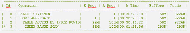
Listing 2: Single Block Read, same statement as above
Distribution of activity
This type of partitioning is aimed at removing bottlenecks. A simple example would be an insert of a large set of rows. In principle a table in Oracle is written to starting with the first data block that holds free space. Now, if e.g. records are written with high frequency, the activity can be concentrated dominantly on one data block. The structures of this block (e.g. transaction slots, block dictionary) might then be overloaded. Contention and similar wait events may occur. Hash partitioning (see corresponding chapter below) can help to prevent this.
Organization of the life cycle of data
Data can go through a life cycle during their existence. The phases of the life cycle can be very different depending on the business processes. A simple example would be the phases of a data record such as "open", "processed", "historical" and "to be deleted". If you map such phases using separate partitions, you can, for example, move historical data to a slower but cheaper storage medium and use a high compression ratio. This takes advantage of the database's ability to store individual partitions in different ways. Obsolete partitions could simply be removed by a drop partition statement, a very efficient way of deleting data. This makes sense, since deleting is the most resource-consuming type of DML.
Partitioning types and typical applications
Range Partitioning

Figure 1: Symbolic representation of range partitioning
Range partitioning is the oldest type of partitioning and the most widely understood. Mostly the range partitioning is associated with a partitioning by date values. But basically, you can partition on every column that is sortable. This can be just as well numbers or alphabetic values. Nevertheless, the classic remains the partitioning by date. This is not surprising because in the first data warehouses, sales data and statistics were the biggest tables and they were usually date related.
If, for example, you want to check whether partitioning by month makes sense for a sales table, you should ask yourself the following questions:
- do most of my queries have a temporal focus?
- what is the most popular temporal focus of most of my queries?
- how old is data that is no longer queried on regular basis?
- are there queries that have no time reference at all, and which are they?
- how long do I have to keep my data?
Here are a few typical answers:
- yes
- last three months
- older than 2 years (previous year comparison)
- sales statistics of a specific customer
- 10 years
Based on the answers above, there would be no reason not to partition the data by the month of sales. The last three months can be found accurately, also the comparison with the previous year would work well. The sales statistics for a particular customer are anyway not searched with a full scan on the partition, but with an index on the customer id. Thus, partitioning is irrelevant with respect to the question. Data older than two years should be compressed as much as possible and considered to be moved to a cheaper storage medium. Partitions older than 10 years I could just drop.
Of course, decision making is not always that easy and sometimes you must weigh the pros and cons. However, it is often possible to find reasonable compromises.
Hash Partitioning
Basics
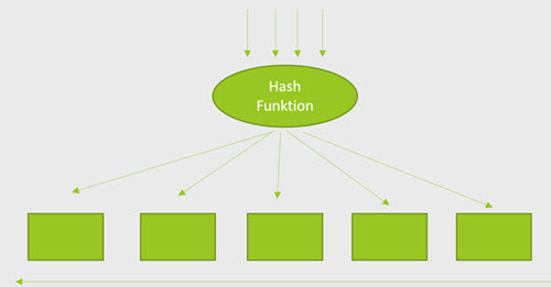
Figure 2: Symbolic representation of Hash Partitioning
Hash partitioning is nothing more than distributing the data sets as evenly as possible over different buckets. Basically, you must only decide how many buckets you want to have and according to which column data should be distributed. The partition key will usually be a primary key or a foreign key. The rest is done automatically by the database and the records are distributed according to the chosen criteria. The hash partitioning normally has no business meaning but optimizes data access and maintenance. Usually, the distribution of activity is targeted to avoid a bottleneck.
Here is an incomplete list of wait events that can be mitigated by hash partitioning:
- Global Cluster waits [4]
- enq: TX - Index contention
- latch: cache buffers chains [5]
- buffer busy waits [3]
I want to mention, that when the partition criteria is non unique, data also gets clustered somewhat by the partition key. It is a statistical and not a perfect clustering, but it still can reduced the I/O to some extent, when the partition key is used in an indexed search.
Example: Partition wise Join
Hash joins can become very large and very memory intensive. If the PGA memory cannot hold the processed data, it must be written on temp tablespace. One way to perform large hash joins more efficiently is the partition wise join. As a prerequisite, the tables that are to be joined must be hash partitioned according to the same criterion. For example, the tables order and order_item. In both tables the column order_nr could exist, in one case as primary key and in other case as foreign key. If you now partition both tables on the order_nr with the same number of hash partitions for each table, corresponding partitions would exists in both tables. For example, the first partition of the order table would contain all records that match the first partition of the order_item table. Instead of joining the whole table, it would be good enough to join corresponding partitions one after the other. This saves resources, i.e. PGA memory and temp tablespace. The figures below document a real case. First, we tried to join both tables as a whole. In Figures 3, we see two loops over all partitions each featuring a storage full scan (the hardware was an Exadata). Figure 4 shows an increasing temp tablespace consumption for 40 minutes. After that, we see a sharp drop in reserved temp space with a peak at about 65 GB. At this point, processing crashed because the temp space was exhausted.
Figure 5 shows the second attempt, this time with a partition wise join. Here you see one hash join nested in a loop over all partitions. The tempspace usage peaks at a comparatively paltry 67 megabytes, which is about one-thousandth of the previous usage. The runtime is 25 minutes and the query finishes this time.
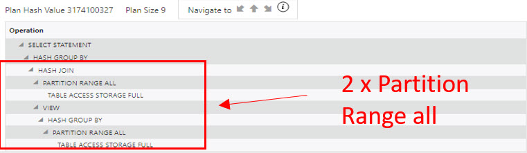
Figure 3: Plan section of SQL Monitor, join of two large tables
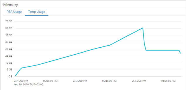
Figure 4: Temp Tablespace consumption increases until crash after 40 minutes of runtime
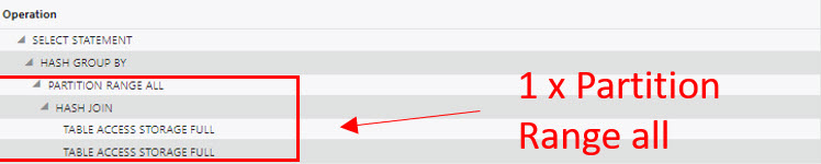
Figure 5: the exact same join as above as partition wise join
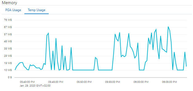
Figure 6: temp consumption of the partition wise join
List Partitioning
Basics
List partitioning assigns a unique value or a list of unique values to each partition. List partitioning can be seen as a special form of range partitioning, but it is shorter to write and clearer in its intent. In practice, I have found that list partitioning sometimes produces subtly better plans than equivalent range partitioning.
Example: Partition by processing status
For a very large customer, documents are to be converted into various (e.g., PDF, HTML) formats according to a set of rules. The decisive factor here is the processing status. When new documents are loaded, the status is initially set to "not processed". After the documents have been converted to different formats, the status is set to "processed". The customer has two issues with the current situation. On the one hand, finding records that have not been processed takes too long, and on the other hand, deleting processed records after the end of the retention period suffers from constant locking problems. My suggestion was to split the data into two partitions. Namely, into "processed" and "not processed" records respectively. The focus of this application was to find "not processed" records. By splitting the data into two partitions, the resources are more focused on the data sets that are of central interest for processing. Take the buffer cache for example. Before partitioning, one block of the buffer cache contained processed and unprocessed records. Thus, if you search for unprocessed records, half or more of the records in a block may be unusable with respect to the search. On the other hand, if all processed records are immediately moved to another partition, the freed space can be claimed by new records with the status not processed. This makes better use of the 8 kilobytes of a data block and makes the search more efficient. I call this a "clean room strategy“ in analogy to the term used in chip production. In addition, deleting old data sets from the traffic-cleared "processed" partition is much easier. However, before you can introduce such a design change, you need to back it up with testing. In particular, the following questions must be answered:
- is the status queried for all relevant queries?
- can the records be moved to the "processed" partition at the same transaction as the status change, or must there be a maintenance process later on?
The partition criteria exists in all queries?
You always have to ask yourself this question before partitioning. Indeed, in this case some queries had to be adapted. In addition, one will often find some queries in which the partition criterion is not contained, then one must ensure that these queries are uncritical with respect to runtime.
Row movement enabled?
The question of potential side effects is also one of the questions that must always be asked with regard to physical database design. One question that arises at this context is, whether records whose status value is changed should be moved immediately to the correct partition or whether this move should be delayed. Technically it means if the value "enable row movement" should be set for this table [6]. If "enable row movement" is set, it means that the record is deleted at the old place and inserted again at the new partition. And this is done in the context of the current transaction. So the records can always be found in just one clearly defined partition. This causes certain overhead, since we are speaking two DML operations (delete, insert) instead of one (update). From experience I can say that this overhead is acceptable, if one record is processed at a time. However, if we are dealing with a mass update, in which records are perhaps also changed in parallel with high frequency, then this overhead will be very disturbing. Thus, the question is whether such a mass update will occurs regularly in the course of standard processing, or whether it will be an exception. You can probably live with an exception, as you can disable the row movement for a short time. If mass updates occur regularly, the row movement must be forbidden, and processed data sets must be stored in the "processed" partition awaiting a dedicated maintenance operation. Although most of the rows that have been processed will still be found in the "processed" partition, the advantages of the clean room strategy defined above will only be partially available.
Reference Partitioning
Basics
As already shown in the partition wise join example above, you can partition two tables in the same way, if the partition criterion is present in both tables. But this is not always the case. If you still want to partition via the same criteria, the missing column needs to be added to one of the tables. However, it is often difficult to talk a software vendor into table definition change. In such case Reference Partitioning might come to rescue.
Reference Partitioning allows for two tables to be partitioned the same way, even if the partition criterion is in only one of the two tables. The precondition is however that the relation between both tables can be established over an active Foreign Key (=reference) constraint.
Example: In-basket processing
In this example I discuss a type of processing for which I did not know an optimal solution until recently. This is the only case in this article where the solution shown has not been tried in the real world. It bases on a test case on my own database. The basic idea is to use reference partitioning to propagate a clean room strategy from one table to another. First a few words about the in-basket (naming by me) problem in general. This task occurs frequently in business processes and reflects a fundamental problem of the delegation of labor. You will not always observe a performance issue with an in-basket situation though. As often in performance optimization size matters. So what does basically define an in-basket set up? From an in-basket a agents fetches his next task to be processed. Such in-boxes can appear at different places in applications. Examples are call center (next call), credit assessment and release, check of insurance claims, order release in manufacturing and many more. The challenge of finding the next task to be processed is that several search criteria have to be combined, which are located on different tables.
Such search criteria can be for example:
- the status of the task
- the knowledge needed to process the task (for example, by assigning it to a specialized group of employees)
- the priority of the order
Below you can see a simplified example of an in-basket. (An important simplification is that it searches directly for a user number and not for a specialist group). You will now be guided through the solution step by step.
Let's start with the basic data structure. In the example we will deal with a call center. The table call lists the calls in the order of arrival. The table is assignment connects calls to users who could potentially take them.
create table call (call_id number(7) not null,
             is_open           char(1) not null,
             priority          number(2) not null,
             data              varchar2(600))
/
create Table Assignment (call_id number(7) not null,
                   user_id number(7) not null,
                   assignment_sequence number(1) not null,
                   data         varchar2(200))
/
create Index assignment_idx1  on assignment(call_id);
Listing 3: DLL for In-basket Example
The following query searches the first ten unanswered calls for user_id 55 sorted by priority.
SELECT * FROM (
SELECT c.call_id, c.data c_data, a.data a_data
  FROM call c,
       assignment a
WHERE c.call_id = a.call_id
  AND a.user_id = 55
  AND c.is_open = 'Y'
ORDER BY priority
)
WHERE rownum <= 11
/
Listing 4: main query to be optimized
The runtime statistics for the query show the actual resources used by the database . Please notice that 17220 records had to be read from the Assignment table to finally have 11 records for the result. That's not very efficient, is it?
-----------------------------------------------------------------------------------------------------------------------------
| Id  | Operation                                | Name          | Starts | E-Rows | A-Rows |   A-Time   | Buffers | Reads  |
-----------------------------------------------------------------------------------------------------------------------------
|   0 | SELECT STATEMENT                         |               |      1 |        |     11 |00:00:03.81 |   47959 |  43494 |
|*  1 |  COUNT STOPKEY                           |               |      1 |        |     11 |00:00:03.81 |   47959 |  43494 |
|   2 |   VIEW                                   |               |      1 |  17220 |     11 |00:00:03.81 |   47959 |  43494 |
|*  3 |    SORT ORDER BY STOPKEY                 |               |      1 |  17220 |     11 |00:00:03.81 |   47959 |  43494 |
|   4 |     NESTED LOOPS                         |               |      1 |  17220 |   1728 |00:00:03.80 |   47959 |  43494 |
|   5 |      NESTED LOOPS                        |               |      1 |  17220 |   1728 |00:00:03.47 |   46318 |  40417 |
|   6 |       TABLE ACCESS BY INDEX ROWID BATCHED| ASSIGNMENT    |      1 |  17220 |  17220 |00:00:03.24 |   20669 |  37907 |
|*  7 |        INDEX SKIP SCAN                   | ASSIGNMENT_PK |      1 |  17220 |  17220 |00:00:00.47 |    4895 |   4895 |
|*  8 |       INDEX RANGE SCAN                   | CALL_IDX1     |  17220 |      1 |   1728 |00:00:00.22 |   25649 |   2510 |
|   9 |      TABLE ACCESS BY INDEX ROWID         | CALL          |   1728 |      1 |   1728 |00:00:00.33 |    1641 |   3077 |
-----------------------------------------------------------------------------------------------------------------------------
Predicate Information (identified by operation id):
---------------------------------------------------
   1 - filter(ROWNUM<=11)
   3 - filter(ROWNUM<=11)
   7 - access("A"."USER_ID"=55)
       filter("A"."USER_ID"=55)
   8 - access("C"."CALL_ID"="A"."CALL_ID" AND "C"."IS_OPEN"='Y')
Listing 5: Result of the first attempt, 47959 buffers, runtime 3.81 seconds
The next step is to apply the cleanroom strategy. In accordance of the previous example we will list partition by status.
create table call_p (call_id number(7) not null,
             is_open           char(1) not null,
             priority          number(2) not null,
             data              varchar2(600))
PARTITION BY LIST (is_open)
(PARTITION OPEN VALUES('Y'),
PARTITION CLOSED VALUES('N')
)
/
Listing 6: Partitioning the Call Table
-----------------------------------------------------------------------------------------------------------------------------
| Id  | Operation                               | Name            | Starts | E-Rows | A-Rows |   A-Time   | Buffers | Reads
-----------------------------------------------------------------------------------------------------------------------------
|   0 | SELECT STATEMENT                        |                 |      1 |        |     11 |00:00:00.80 |   32615 |  32609
|*  1 |  COUNT STOPKEY                          |                 |      1 |        |     11 |00:00:00.80 |   32615 |  32609
|   2 |   VIEW                                  |                 |      1 |  17220 |     11 |00:00:00.80 |   32615 |  32609
|*  3 |    SORT ORDER BY STOPKEY                |                 |      1 |  17220 |     11 |00:00:00.80 |   32615 |  32609
|*  4 |     HASH JOIN                           |                 |      1 |  17220 |   1728 |00:00:00.80 |   32615 |  32609
|   5 |      TABLE ACCESS BY INDEX ROWID BATCHED| ASSIGNMENT      |      1 |  17220 |  17220 |00:00:00.46 |   15859 |  15856
|*  6 |       INDEX RANGE SCAN                  | ASSIGNMENT_IDX1 |      1 |  17220 |  17220 |00:00:00.04 |      82 |     82
|   7 |      PARTITION LIST SINGLE              |                 |      1 |    100K|    100K|00:00:00.32 |   16756 |  16753
|   8 |       TABLE ACCESS FULL                 | CALL_P          |      1 |    100K|    100K|00:00:00.32 |   16756 |  16753
-----------------------------------------------------------------------------------------------------------------------------

Predicate Information (identified by operation id):
---------------------------------------------------

   1 - filter(ROWNUM<=11)
   3 - filter(ROWNUM<=11)
   4 - access("C"."CALL_ID"="A"."CALL_ID")
   6 - access("A"."USER_ID"=55)
Listing 7: Runtime statistics with partitioned table Call
Things have improved buffers are lower now. However, that cannot be the optimum yet. Too many rows are thrown away still. In the next step, the cleanroom strategy is propagated to the table CALL using reference partitioning.
create Table Assignment_p (call_id number(7) not null,
                   user_id number(7) not null,
                   assignment_sequence number(1) not null,
                   data         varchar2(200),
                   CONSTRAINT pk_Assignment_p primary key
                      (call_id , user_id ,
                       assignment_sequence ),
                   CONSTRAINT callid_ref FOREIGN KEY (call_id)
                       REFERENCES   call_p (call_id)
)
partition by reference (callid_ref )
pctfree 50
/
create Index assignment_p_idx1  on assignment_p(call_id) local;
Listing 8: Reference partitioning of table ASSIGNMENT.
Only now does the partitioning strategy shows its full effect. The runtime drops drastically.
On the positive side, it can be noted that the runtime behavior should remain stable in the future. Even if the number of completed calls increases, the number of open calls will remain approximately constant. In accordance will the effort to retrieve open calls (full partition scan) stay constant as well. This is important to notice, as I have experienced that a growing number of processed rows can otherwise cause execution plans to shift in a negative way, harming performance.
--------------------------------------------------------------------------------------------------------
| Id  | Operation                     | Name         | Starts | E-Rows | A-Rows |   A-Time   | Buffers |
--------------------------------------------------------------------------------------------------------
|   0 | SELECT STATEMENT              |              |      1 |        |     11 |00:00:00.05 |   26112 |
|*  1 |  COUNT STOPKEY                |              |      1 |        |     11 |00:00:00.05 |   26112 |
|   2 |   VIEW                        |              |      1 |  15272 |     11 |00:00:00.05 |   26112 |
|*  3 |    SORT ORDER BY STOPKEY      |              |      1 |  15272 |     11 |00:00:00.05 |   26112 |
|   4 |     PARTITION REFERENCE SINGLE|              |      1 |  15272 |   1728 |00:00:00.05 |   26112 |
|*  5 |      HASH JOIN                |              |      1 |  15272 |   1728 |00:00:00.05 |   26112 |
|*  6 |       TABLE ACCESS FULL       | ASSIGNMENT_P |      1 |  15272 |   1728 |00:00:00.02 |    9360 |
|   7 |       TABLE ACCESS FULL       | CALL_P       |      1 |    100K|    100K|00:00:00.02 |   16751 |
--------------------------------------------------------------------------------------------------------
Predicate Information (identified by operation id):
---------------------------------------------------
   1 - filter(ROWNUM<=11)
   3 - filter(ROWNUM<=11)
   5 - access("C"."CALL_ID"="A"."CALL_ID")
   6 - filter("A"."USER_ID"=55)
Listing 9: Runtime statistics with both partitioned tables and partition wise join
Conclusions
As can be seen, partitioning is a very effective tool making the physical design more efficient. There is no generic rule on how to partition a data model. (Even though people of course wish such rules exists.) For that reason, this article provides practical examples, in the hope of sharpening the reader's eye for options. As a guideline, it is important that the business process is reflected in the design.
There are advantages and disadvantages to many designs. Quite often, one does not come without the other. (“You do not get something for nothing”, as my first design teacher used to say.) Weighing these against each other is the creative effort behind a database design.
About The Author

On February 1st, 1989 I was allowed to take my first steps with Oracle. A lot of time has passed since then. I was an Oracle employee for 15 years and also a member of the Real World Performance Group. I'm an Oaktable Member and an Oracle ACE. I have a patent to improve the optimizer and worked on the software for the LHC at CERN in Geneva. Today I am an employee of DBConcepts GesmbH in Vienna.
References:
- [1] Get the best out of Oracle Partitioning, Online Guide
- [2] Wikipedia, Partition (database)
- [3] Hesse, Uwe, How to reduce Buffer Busy Waits with Hash Partitioned Tables in #Oracle
- [4] Riyaj Shamsudeen, gc buffer busy waits
- [5] Author probably Kyle Hailey, Oracle: latch: cache buffers chains
- [6] Hemant K Chitale, ENABLE ROW MOVEMENT
- [7] Dani Schnider, Housekeeping in Oracle: How to Get Rid of Old Data